zkML for =nil; Proof-Market

Approximately six months ago, we announced our collaboration with =nil to introduce (zkML) to the =nil Proof-Market. Since then, we've been diligently working on developing an ONNX extension for zkLLVM, and today, we're thrilled to share our progress with you. This tutorial will walk you through the process of compiling an ONNX model into an intermediate representation, generating a circuit and an extended witness from the intermediate representation, and creating a proof from the circuit and the extended witness. Additionally, we'll provide a brief overview of the zkML workflow and demonstrate how to use our zkML compiler and assigner to generate a proof from a Random Forest model with private inputs.

If you're keen to delve deeper into the intricacies of our solution, feel free to explore our announcement blog post here. Depending on how things unfold in the future, we may also consider writing a more detailed blog post about the technical aspects of our solution, so stay tuned for updates!

Disclaimer

This tutorial was written in February 2024. The software and libraries used are still under active development, and the commands and flags may change in the future.

Setup and Build

Alright, let's get started. Before we can begin proving anything, we need to set up a few things. In this section, we'll walk through the steps to set up and build the procedure for proving ONNX models. First and foremost, you'll need to obtain the source code from the repository. You can clone the repository using the following command:

git clone --recurse-submodules -j 8 https://github.com/TaceoLabs/zkllvm-mlir-assigner

Executing this command will clone both the repository and its submodules. The '-j 8' flag is employed to accelerate the cloning procedure by utilizing 8 threads concurrently. Once the repository is cloned, the subsequent step involves building the project. Given that one of the dependencies is ONNX-MLIR, which relies on MLIR/LLVM, building these projects from scratch can be cumbersome. To streamline this process, we've prepared a Nix developer shell . Accessing the Nix shell can be accomplished by executing the following command (inside the zkllvm-mlir-assigner directory):

nix develop --cores 8

We allocate 8 cores to fasten the build process, particularly crucial for compiling LLVM (throw as many cores at the problem as you want). Given the time-consuming nature of this task, it's a good opportunity to take a break – perhaps enjoy a cup of coffee or delve into topics like ZK-friendly hashing or MPC, which are among our favorites.

Once inside the Nix shell (and one coffee later ☕), executing the following commands will initiate the project build:

mkdir build && cd build && cmake -DMLIR_DIR=${MLIR_DIR} .. && make -j 8 zkml-onnx-compiler mlir-assigner

You now find two binaries in the build directory: zkml-onnx-compiler and mlir-assigner.

A Toy Example

Congratulations on successfully building the project! Now, let's delve into a straightforward example to demonstrate the workflow. Our objective is to acquire both the circuit representation of the model and the extended witness, which comprises the assigned table.

To achieve this, we'll utilize the zkml-onnx-compiler to compile the ONNX model into an intermediate representation (MLIR). Subsequently, we'll employ the mlir-assigner to generate the circuit and the witness from this intermediate representation.

You can locate the model in the examples/ directory. To simplify matters, let's begin by copying the two binaries into the examples/ directory:

cp build/bin/* examples/ #copy the zkml-onnx-compiler and mlir-assigner to the examples directory
cd examples/

Within the examples/ directory, you'll find the toy example located in the addition/ directory, along with a sample input. We recommend to use the amazing application netron to inspect ONNX models. The toy example that we inspect is a simple addition of two $1\times 10$ tensors, which looks like this:

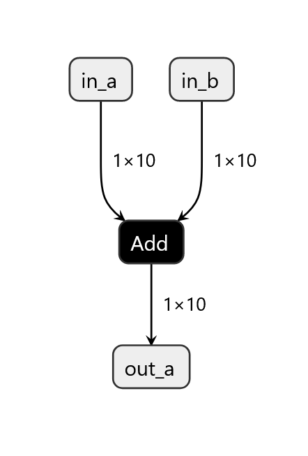
Figure 1: The structure of the toy example

Before proceeding with compiling the ONNX model into MLIR, it's crucial to address a significant aspect of this process. Specifically, we must specify whether we intend to enforce the Zero-Knowledge property for certain (or all) inputs. In our current example, we designate the first input tensor as private, while the second one is marked as public. This scenario mirrors real-world situations where, for instance, one input may contain confidential model weights. To specify the privacy of the inputs, we utilize the --zk flag, which accepts a comma-separated list of 0s and 1s. Each input marked with 0 will be considered public, while those marked with 1 will be treated as private. In the toy example the command looks the like this:

For that we execute the following command:

./zkml-onnx-compiler addition/addition.onnx --zk 1,0 --output addition/addition.mlir

The compiler writes the MLIR representation of the ONNX model to the file specified, in our case this is addition/addition.mlir. When inspecting the model in the MLIR format, you'll notice that the first input tensor is marked as private, as specified in the command (we skip this for brevity, but feel free to challenge us on our words and have a look yourself).

Next, we need to prepare the input for the mlir-assigner. We have two input files, one for the public input and one for the private input, both are in JSON format. The private input file for our example looks like this:

[
  {
    "memref": {
      "idx": 0,
      "data": [
        -9.0, -9.887, 4.543, -3.75, 2.743, 5.43, 1.87, -5.65, 0.564, -3.2345
      ],
      "dims": [1, 10],
      "type": "f32"
    }
  }
]

Let's examine the structure of this JSON file. The memref object comprises the following fields:

• idx: This denotes the index of the input tensor in the MLIR file. In our case, the first input tensor has an index of 0. It's important to note that the idx applies only to private inputs; for public inputs, the idx restarts from zero.
• data: This field contains the flattened data of the input tensor.
• dims: Represents the dimensions of the input tensor.
• type: Specifies the data type of the input tensor. In our examples, we utilize f32 for floating-point numbers. Other potential values include int for integers and bool.

Each input file, whether private or public, must encompass a list of memref objects, each adhering to this structure. For brevity, we omit details regarding the public input file, as it shares the same structure as the private input file. With this setup complete, we can proceed to generate the extended witness and the circuit using the following command:

./mlir-assigner -b addition/addition.mlir -i addition/public.json -p addition/private.json -o addition/addition.out.json -c addition/addition.circuit -t addition/addition.table -x 16.16 -e pallas -f dec

Upon executing this command, you should observe the following output:

Result:
memref<1x10xf32>[-5.68001,-7.58701,-1.81699,2.78,-6.507,0.559998,-1.66,-2.55,11.564,3.2655]
20 rows

This output provides a human-readable representation of the addition operation result, facilitating verification or understanding of the model output. Moreover, the binary generates an output file at the designated location specified by the -o flag. In our scenario, this file is located at addition/addition.out.json. Furthermore, it's worth noting that the output file is also constrained within the circuit.

As for the other flags, lets examine them in detail:

• -b: Specifies the path to the MLIR file.
• -i: Indicates the path to the public input JSON.
• -p: Denotes the path to the private input JSON.
• -o: Specifies the location for writing the output file.
• -c: Specifies the location for writing the circuit.
• -t: Specifies the location for writing the assigned table (the extended witness).
• -x: Specifies the fixed-point format size for the model evaluation.
• -e: Specifies the elliptic curve used. At present, we recommend using pallas.
• -f: Specifies the format of the printed result. In our case, we utilize dec for decimal. This flag can also be omitted.

Check the --help flag for both binaries to get more information about the flags. Anyways, that is as far as we go with the toy example. Now that we have the basics down, we can move on to more complex examples.

Convolution based MNIST

Let's continue this time with a real model. The MNIST model is a classic example in machine learning, focused on recognizing handwritten digits from 0 to 9. It employs a convolutional neural network (CNN) architecture to extract features from 28x28 pixel grayscale images and classify them. You can find the model at examples/mnist/mnist-12.onnx. Inspecting the model in netron, we can see the structure of the model:

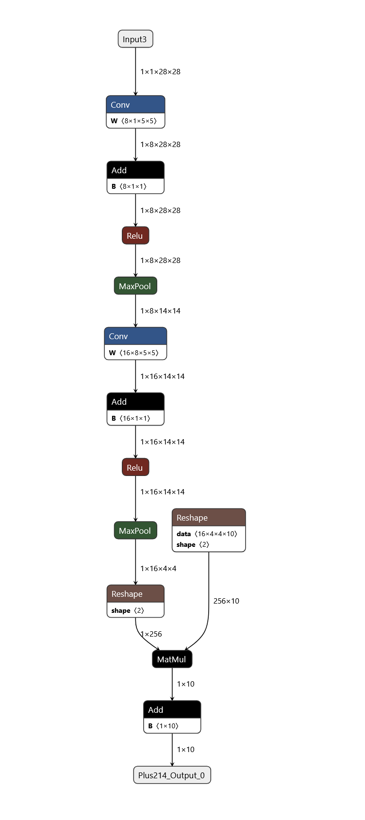
Figure 2: The structure of the MNIST model

Circuit and Witness Generation

Next to the model you can find a sample input in the examples/mnist/ directory. The input is a 28x28 pixel grayscale image of the digit 1. As learned from the toy example, we can compile the model into MLIR using the zkml-onnx-compiler:

./zkml-onnx-compiler mnist/mnist-12.onnx --zk 0 --output mnist/mnist-12.mlir

After that we can use the mlir-assigner to generate the circuit and the witness from this intermediate representation:

./mlir-assigner -b mnist/mnist-12.mlir -i mnist/public.json  -o mnist/mnist-12.out.json -c mnist/mnist-12.circuit -t mnist/mnist-12.table -x 16.16 -e pallas -f dec

You should get the output that's look similar to this:

Result:
memref<1x10xf32>[23.1523,-17.667,4.46326,-9.95807,-3.84666,-2.20348,3.83511,-9.20743,-2.53932,-0.523529]
178640 rows

Since the highest number in the first position of the result corresponds to the predicted digit, which is 1 in this case, we can infer that the model correctly identifies the input. The execution of this model may have taken a few seconds due to the computational cost associated with convolutions and matrix multiplications, which are resource-intensive operations within the circuit. During the conversion process from ONNX to MLIR, it's possible to annotate the model with debug information. This can be achieved by appending the --DEBUG flag, as follows:

./zkml-onnx-compiler mnist/mnist-12.onnx --zk 0 --output mnist/mnist-12.mlir --DEBUG

Rerunning the mlir-assigner with the command as before, you will notice that there will be additional output to indicate the progress of the circuit and extended witness creation.

Creating the Proof

We stopped at this point with the toy example but now we press forward. So far we only created a circuit from a model and an extended witness from a concrete input. The next step is to create a proof from the circuit and the extended witness. This is done using =nil;'s Proof Producer¹. After installing the proof-producer, we can create a proof using the following command:

proof-generator-multi-threaded --circuit mnist/mnist-12.circuit -t mnist/mnist-12.table -p mnist/proof.bin -e pallas

Depending on your machine, this process may take a minute, but it shouldn't be excessively long. The proof is saved to the file specified by the -p flag, which in our case is mnist/proof.bin. As previously mentioned, you must specify the circuit, the table, and the elliptic curve used.

A Random Forest with Private Inputs

Now, having demonstrated how to generate a proof from the MNIST model, let's explore creating a proof from a model relevant for DeFi applications: a Random Forest. A Random Forest is a highly adaptable ensemble learning technique employed predominantly for classification and regression tasks in machine learning. It functions by constructing multiple decision trees during training, with each tree trained on a random subset of the training data and features. During prediction, the Random Forest aggregates the predictions of each individual tree to produce a final prediction.

We prepared a Random Forest model for this example, which is located at examples/random-forest/random-forest.onnx². In this scenario, we'll assume that the input to the model is confidential.

Now that we are experts already, we go through the steps a little bit faster. We compile the Random Forest, and specify the input as private (for tracing remember the --DEBUG flag):

./zkml-onnx-compiler random-forest/random-forest.onnx --zk 1 --output random-forest/random-forest.mlir

We generate the circuit and the witness:

./mlir-assigner -b random-forest/random-forest.mlir -p random-forest/private.json  -o random-forest/random-forest.out.json -c random-forest/random-forest.circuit -t random-forest/random-forest.table -x 16.16 -e pallas -f dec

You should see the following output:

Result:
memref<1xf64>[0]
29239 rows

To create the proof, we use the following command:

proof-generator-multi-threaded --circuit random-forest/random-forest.circuit -t random-forest/random-forest.table -p random-forest/proof.bin -e pallas

Conclusion

We've reached the end of this tutorial. We hope you found it helpful! If you have any questions, suggestions, or feedback, don't hesitate to reach out to us on Twitter or via the GitHub page of the project. We're always eager to assist and learn from your experiences. We're excited to see what you'll create with zkML and the =nil; Proof-Market.